This post was written and submitted as part of an entry into RStudio’s Table Contest: 2021 Edition. If you’re not interested in an R tutorial, check out any of our other posts or just read the beginning and the end to get an idea of what we’re doing with track & field results data.
No one has ever accused track & field of being fan friendly. Even fewer people have accused track & field results of being fan (or data scientist) friendly. Although, tbf, not many sports fans nor data scientists go looking for them.
But for the last 10 years, George has been con-VINCED that he can do something with, or at least in, this sport. And things took an interesting turn when he found Greg – data scientist, swimmer and creator of SwimmeR and JumpeR – last summer.
In this tutorial, we’ll take a break from swimming, running and jumping to walk through how we combined JumpeR, Shiny, reactable and gt to produce informative, interactive and pleasant results tables for athletes in the vertical jumps of track & field: pole vault and high jump.
Making track & field data useful with JumpeR
Track & field result sheets manage to provide a lot of information without actually telling you anything. High jump and pole vault results usually come out looking something like this:
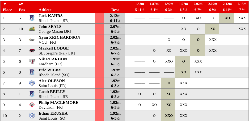
Or even this:
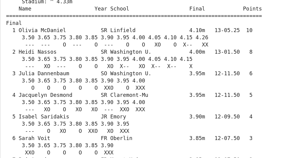
Sadly, not only is that what goes in the official record of the meet, it’s usually what makes its way onto websites and social media. On meet days, photos of printouts and screen caps abound on T&F Twitter and Insta. Results are scattered all over the web, so simply compiling a bunch of these results sheets is quite challenging, let alone if you wanted to get a snapshot of an athlete’s season or career. “How many heights did she clear at last year’s national championships?” is a question few ask, and no one other than the athlete and her coach could probably answer.
Enter JumpeR. JumpeR is built using many tools from rvest and some functions from SwimmeR.
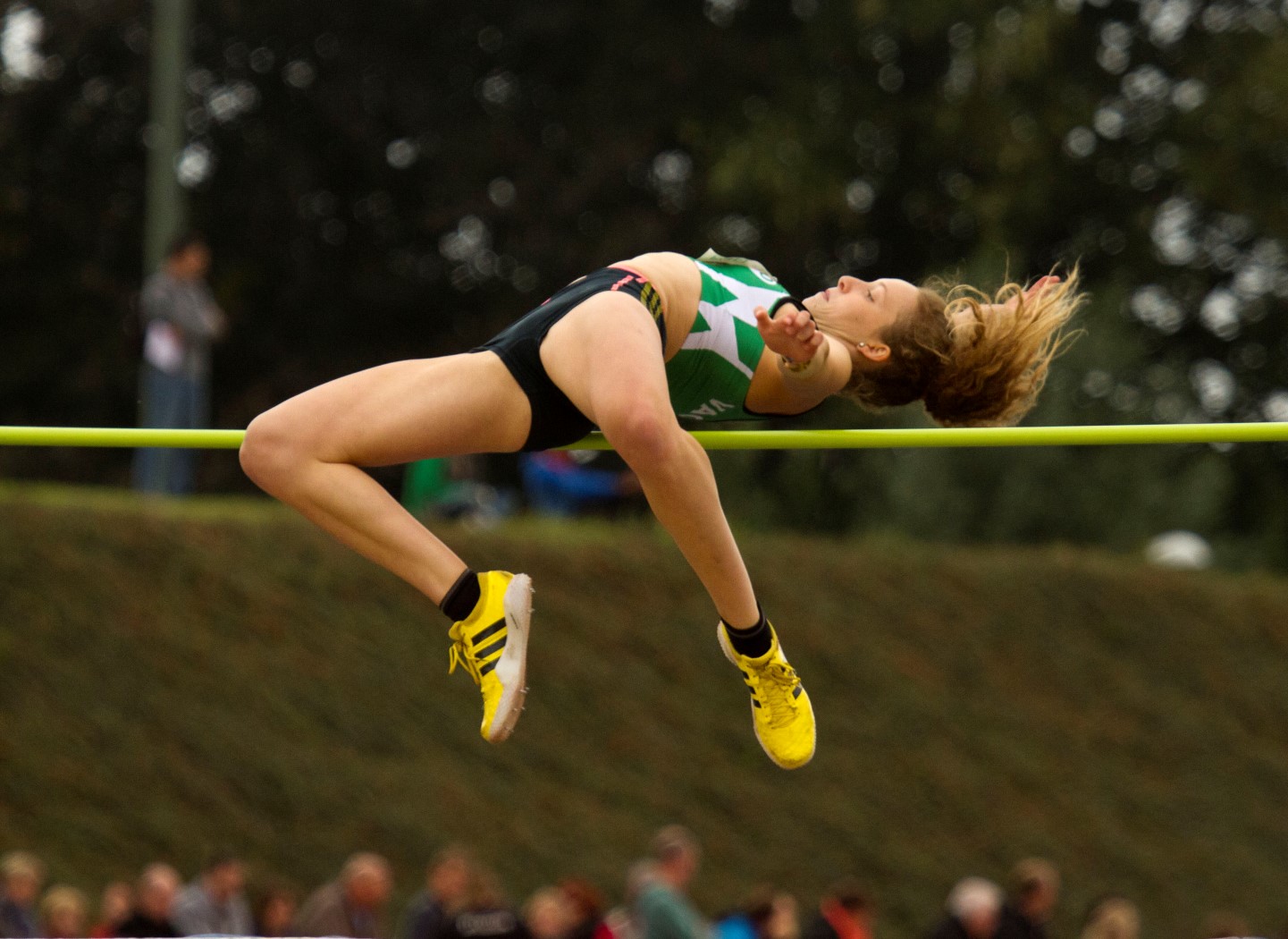
JumpeR can handle nearly any format of track & field results, and all of the events within track & field. Shot put - where each athlete gets six throws - and the 100m dash will obviously have different outcomes and, therefore, different results formats. Among the vertical jumps, each meet will have a different number of heights: the bar starts at given level, each athlete has 3 chances to clear it. If they can’t, they’re out. The bar goes up a few centimeters in each round until no one can get over it. This aspect of the sport will be crucial later on.
We used JumpeR to pull down several years worth of high school, collegiate and professional track & field results data. JumpeR’s output is readily displayed in a wide format – similar to what comes out on the sheet – and is easily converted to a tidy “long” format.
The tables we sketched out required a bit of follow-on processing. After getting everything into a very long, very tidy format, we got to work on creating new metrics for the sport. For each meet an athlete competes in, we wanted to present a “box score” of not just her mark, but how many different heights she attempts to clear, how many of those heights she cleared, how many jumps she took and how many of those were successful. This required a lot of group_by and ungroup as the new and old metrics required us to compare the athlete against herself and against her opponents at each meet.
vertical_championships %>%
  pivot_longer(cols = contains("Attempt"), names_to = "Attempt", names_prefix = "Attempt", values_to = "Outcome") %>%
  filter(Outcome == "O" | Outcome == "X") %>%
  select(Name, Meet, Event, Gender, Height, Bar_Order, Event_Date, Attempt, Outcome, Meet_ID, Event_ID) %>%
  group_by(Name, Event, Event_Date, Outcome) %>%
  mutate(Meet_Mark = case_when(Outcome == "O" ~ max(Height),
                               TRUE ~ NA_real_)) %>%
  ungroup() %>%
  group_by(Name, Event, Event_Date) %>%
  mutate(Meet_Jump_Attempts = length(Outcome),
         Meet_Ht_Attempts = length(unique(Height)),
         Meet_Ht_Clear = sum(Outcome == "O"),
         Meet_Jump_Clear = Meet_Ht_Clear) %>%
  ungroup() %>%
  filter(Meet_Mark != "NA") %>%
  group_by(Event, Gender, Event_Date) %>%
  mutate(Place = match(Meet_Mark, sort(unique(Meet_Mark), decreasing = TRUE))) %>%
  ungroup() %>%
  distinct(Name, Event, Meet, Gender, Meet_Mark, Place, Event_Date, Meet_Ht_Attempts, Meet_Ht_Clear, Meet_Jump_Attempts, Meet_Jump_Clear, Meet_ID, Event_ID)
Structuring with Shiny (although that won’t be all)
We want fans to be able to engage with the athletes via data, so of course we started with Shiny. The only input we need to get started is an athlete’s name. Below that is an area for the athlete’s name and event, and then the two tables. Clean, vertical, mobile-friendly.
ui <- fluidPage(
         tags$head(includeCSS("www/vertical_tables.css")),
         useShinyjs(),
                fluidRow(
                  column(12,
                      selectizeInput("Name_rt", choices = NULL, label = "Find an athlete") %>%
                        tagAppendAttributes(class = "athlete_input"),
                      hr()),
                  column(12,
                      textOutput("athlete") %>%
                        tagAppendAttributes(class = "athlete_name_big"),
                      textOutput("event") %>%
                        tagAppendAttributes(class = "athlete_event_big")
                      ),
                   column(12,
                      reactableOutput("name_rt"),
                    hr(),
                    gt_output("gt_meet"))
                    )
Once an athlete is selected, we use her name to filter our partially-processed results data for all the meets she competed in. We then extract the event she competes in. Since our results contain decathletes and heptathletes – the only ones crazy enough to compete in both high jump and pole vault – if the athlete competes in more than one event, we note them as a Multi athlete. Now we have Name and Event, which goes into the top of the page.
reactable: Creating a table of box scores for every pole vaulter and high jumper
Reactable offered three key features for our first table.
1. Column groups
Our results summary will contain the number of bar heights each athlete attempts and complete, and the number of total jumps the athlete attempts and completes. These are pretty lengthy column titles, and since these are new metrics, we didn’t want to abbreviate them as “AJ” for attempted jumps, and so on. They are also very similar: attempts and clearances for one, and the other.
Which means they are perfect grouping.
We define our columns within our renderReactable call, but before we start creating the table itself. Then, in the reactable() call, we define columnGroups using the names we gave those vectors, and then give them their obvious names.
output$name_rt <- renderReactable({

    #### columns for bar heights and number of jumps ####
  agg_height_cols <- c("Meet_Ht_Attempts", "Meet_Ht_Clear")
  agg_jump_cols <- c("Meet_Jump_Attempts", "Meet_Jump_Clear")

  ...


columnGroups = list(
                  colGroup(name = "Heights", columns = agg_height_cols),
                  colGroup(name = "Jumps", columns = agg_jump_cols)
                )
One thing to watch when creating grouped columns is that you create two different elements in the table’s header. You can style these using headingStyle or groupHeadingStyle. But since we already had a CSS stylesheet going, we customized the background color and font color by accessing the header groups.
.rt-thead, .rt_header_class {
    color: #fefefe;
    background-color: #2d4268;
}
2. Footer row
The footer row in a reactable table is not unlike using summarize in dplyr: you can take the sum, mean or any other aggregate function on the column. But how you do it is different.
Footers can be text, a calculated value or some combination of the two. If the footer for a cell is an aggregate function, it’s given as a function of the values in a column and the name of a column. Any of this can be done within the colDef for a given column.
columns = list(
                  Meet = colDef(minWidth = 85, align = "left", footer = "Average per meet:"),
But we’re doing the same thing – taking the sum - to 4 of our columns, and we didn’t want to add the same line of code to the colDef for those 4 columns. Instead, we used the defaultColDef, but made it less-than-truly-default by having it apply only to those columns that show attempts or clearances.
 defaultColDef = colDef(align = "center",
                                       headerClass = "rt_header_class",
                                       footer = function(values, name)
                                         if (str_detect(name, "Attempts|Clear")) {
                                           col_summary <- round(sum(values) / length(values), 1)
                                           return(col_summary)
                                         }
                                       ),
3. Sorting and selection
This is where reactable is just plain cool. Clicking on any column heading will sort the table on the values of that column. We went back to the stylesheet to make the selected column heading appear in a yellow box with a black font, so you can see at a glance what column the table is sorted on. We also set defaultSorted = “Meet_Mark”, so the table would be sorted upon arrival by the single most important and familiar metric from a meet; and so visitors would recognize that the table is, in fact, sortable.
.rt_header_class[aria-sort="ascending"],
.rt_header_class[aria-sort="descending"] {
  background-color: #faff43;
  color: #040000;
}
By setting selection = “single”, we give visitors the option of selecting a row corresponding to a meet. We used the theme property to make the selected row more noticeable: coloring the background and adding a little red bar on the left side.
theme = reactableTheme(
                  rowSelectedStyle = list(backgroundColor = "#cbdeff", boxShadow = "inset 5px 0 0 0 #ff180e")
                )
But the real action lies beneath.
gt is ready for the uncertainty of track & field meets
It would be a pretty common fan behavior to want to know the full details of one or two of the meets. Maybe that’s the meet they visited the page to see, or maybe something about the box score caught their eye and now they want the full picture.
By selecting the row, they can get the full meet results. Easy, right? Not so fast.
reactable is great, but we encountered a limitation. Column groups have to be defined explicitly in reactable. This was easy enough earlier, because we knew the column groups we wanted. But remember what we said up towards the beginning: each meet has a different number of heights, and the heights are different from one meet to the next. Not only can you not define the names of the column groups you need, but you don’t even know how many you need.
We could have used a for loop over the number of heights in the meet to add columns as necessary and then populate their names. But c’mon, it’s 2021 ffs, we’re not doing a for loop. Not when we have gt.
gt has tab_spanner_delim(). This function takes in column names and splits them into spanner column headings and column headings based on a delimiter in the column names. No need to define the column names explicitly, no need to know how many columns you need.
Game-changer. Er, meet-changer.
But first, we would need to get our data into a format where tab_spanner_delim can do its thing. We know we want the spanner columns to be the height, and the columns to be the outcome of each attempt.
Oh, and we want the rows to be ordered in the order in which the athletes finished:
 full_meet_table <- reactive({
    full_meet <- vertical_championships %>%
      filter(Event_ID == selected_meet()) %>%
      select(Name, Attempt1, Attempt2, Attempt3, Height, Meet_ID, Event_Date, Event, Gender) %>%
      pivot_longer(
        cols = contains("Attempt"),
        names_to = "Attempt",
        names_prefix = "Attempt",
        values_to = "Outcome"
      )

    #### order athletes by finish place ####
    standings_order <- full_meet %>%
      filter(Outcome == "O" | Outcome == "X") %>%
      group_by(Name, Outcome) %>%
      mutate(Mark = case_when(Outcome == "O" ~ max(Height),
                              TRUE ~ NA_real_)) %>%
      ungroup() %>%
      group_by(Name) %>%
      mutate(Attempts = n()) %>%
      distinct(Name, Mark, Attempts) %>%
      arrange(desc(Mark), desc(Attempts)) %>%
      filter(!is.na(Mark)) %>%
      select(Name) %>%
      as.vector()

    #### vector to arrange table - order of finish ####
    table_order <- as.vector(standings_order$Name)

      full_meet %>%
      arrange(factor(Name, levels = table_order)) %>%
      mutate(Bar_Attempt = paste0(sprintf("%.2f", Height), "_", Attempt),  # Creates column names that tab_spanner_delim can split
             Outcome = case_when(is.na(Outcome) ~ " ",
                                 Outcome == "" ~ "  ",
                                 TRUE ~ Outcome))  %>%
      select(Name, Outcome, Bar_Attempt) %>%
      pivot_wider(names_from = "Bar_Attempt", values_from = "Outcome") %>%
      mutate(across(matches("^\\d"), ~replace(., is.na(.), "   "))) %>%
      mutate(across(cols = -Name, .fns = ~ as.factor(.))) %>%
      select(!matches("^\\d"), str_sort(names(.), numeric = TRUE))
Since we want the table to be informative and visually pleasant, we know it can’t just be a garble of X’s, O’s and -’s and P’s (those last two are when an athlete passes on a jump or height). There should be some easy to understand color scheme: red for a miss, green for a clearance and an unobtrusive but distinctive blue for a pass seems logical, right? We define this before we start building the table. Then, once we’re in the table, we then rely on gt’s close relationship with htmltools to set the data_color.
color_scheme = c(X = "#ff180e",
                 O = "#44aa22",
                 P = "#cbdeff")
    ...
data_color(
    columns = -Name,
    colors = scales::col_factor(
    palette = color_scheme,
    domain = names(color_scheme),
    ordered = TRUE
        ),
    apply_to = c("fill", "text")
 )
Shiny really ties the room together
But wait a second. You’ve probably already caught on that we’ve skipped something. How did we go from selecting a row in a reactable table to building a gt table based on that row selection?
It was a Shiny day when we made the connection.
Go back up in the code, between the two tables. reactable has a function getReactableState, which does exactly what the name says: it lets you access the state of a reactable instance when using Shiny and reactable together. We pass the name of our table and use the parameter “name” to let the function know we want the name (as opposed to the index) of the selected row.
#### get meet (row) selected in reactable to display detailed results for ####
  selected_row <- reactive(
    getReactableState("name_rt", name = "selected")
    )

  #### meet to display complete, detailed results for ####
  selected_meet <- reactive({
    athlete_selection() %>%
      slice(selected_row()) %>%
      select(Event_ID) %>%
      pull()
  })
The output is just (“just”) a reactive that contains the name of the meet the user selected. We can then use that to get the Event_ID - a value that we kept but did not show in the table - of the meet that we want. The Event_ID uniquely identifies pole vault or high jump, men’s or women’s, and event date of every event in the data. With this in hand, we can easily go back to start manipulating doing the steps we outline above (and a bunch of others) to work towards the gt table.
So let’s pause in appreciation. Shiny and reactable work well together. gt and Shiny work well together. reactable and gt don’t. But we can use Shiny as an intermediary to pass the information we need from reactable to gt, allowing a selection in the former to be an input for the latter.
What’s left to do?
A lot! We know what we have on our to-do list, but a big part why we decided to do this was to get more people than just the two of us to be playing with and exploring track & field (and swimming) data. To that end, all of the results data from championship meets - like what we used in this tutorial - will be available via a public repo by the end of 2021. People can’t have fun with data unless they have the data, and athletics needs all the eyes it can get.
On that note of attention-seeking behaviors, if you’ve read this far you clearly like George and his writing quite a bit and you may have thought to yourself “His writing is way better than his R.” If that’s the case, first off, you’re right. So please check out his recently released book, EGOals: Exercising Your Ego in High-Performance Environments, which he co-authored with sports performance scientist Martin Buchheit. And stay up on all things track & field data at NALathletics.
And if swimming or more serious R chops are your thing, then dive (HA!) into the SwimmeR world with Greg’s website and GitHub page.